In today’s post we will be looking at a couple of ways you can train a self-supervised model to handle variable lists of elements, using vanilla and variational autoencoders.

Code here

Why should I care about sets?

Well it turns out you probably already do care about sets. If you’ve ever calculated an average of an array, or pulled members of a population out that match some definition, you’ve already been solving set problems. These problems are incredibly common, we are just used to dealing with special cases of them.

What even is a set?

Sets have two main properties that define them. The first property of a set is that it is permutation-invariant, aka the elements have no order. This doesn’t mean that there isn’t a structure to the elements, it’s just that this structure is not defined explicitly by the data type. The structure is instead a function of all of the elements. The second property is that a set does not have a fixed size. These two properties pose some interesting challenges for modelling sets both in terms of classification and generation.

An example problem

The experiments in this post are based upon two papers:
TSPN - Adam R Kosiorek, Hyunjik Kim, Danilo J Rezende
Set Transformer - Juho Lee, Yoonho Lee, Jungtaek Kim, Adam R. Kosiorek, Seungjin Choi, Yee Whye Teh

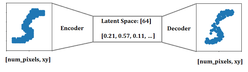
We’ll be looking at the MNIST dataset, but in a slightly different format than what you are probably used to. Instead of treating samples as images, we will be collecting the digit pixels into a set of pixel locations. This gives us a set of coordinates that define the digits. Our goal is to compress these coordinates into a fixed size vector, then see if we can rebuild the original digit.

The code for the MNIST-Set dataset is available here

The Autoencoder Framework

An autoencoder is a self-supervised framework that uses reconstruction as it’s training method. Autoencoders are composed of two models, an encoder and a decoder. The role of the encoder is to model the input information into a vector that contains useful information about the input. The decoder then has to rebuild the original input as closely as it can, using just the encoders output vector. In this case, the autoencoder can be viewed as an information compressor. This is an interesting challenge for sets, as the set size is not constant, yet we are squeezing the set into a fixed sized vector. The decoder also needs to produce a variable sized output, given a fixed sized input.

I won’t go into too much detail about the two architectures because the papers cover them much better than I can, but here is a quick overview:

The model used in the Encoder is called a Set Transformer; this is a generalised version of the classic Transformer used in many language modelling scenarios, but the positional encoding has been removed because our sets are order-invariant. It has an additional layer that uses a Transformer to pool elements together into a single or subset of vectors using learned comparison vectors.

The Decoder uses a model called TSPN (Transformer Set Prediction Network). This builds off the Set Transformer listed above, beginning with a randomly sampled initial set. Each element is conditioned with the latent vector to provide information about the goal output, then the elements are transformed (hopefully) back into the original set.

It turns out that from the encoder output, we can learn a simple model that predicts the set size. This means that we can learn to predict an output set without the input being a set, allowing applications such as image-to-set (where are the faces in this image?), sentence-to-set (what are the emotions in this line?) or any other …-to-set you can think of.

The full code for the AutoEncoder is available here

The Variational Variant

Often with vanilla autoencoders, the latent space ends up being quite sparse. There are regions of high density where the model reconstructions are good, with large areas between where reconstructions are meaningless.

There is an additional type of autoencoder called the variational-autoencoder, or VAE for short, which pushes the model to allow the latent space to be noisy during training, forcing the model to attempt to create good reconstructions from imperfect information. The model needs to trade off between reconstruction loss whilst minimising KL-Divergence. The better it can reconstruct despite imperfect information, the better the it will achieve both goals concurrently.

The benefit of this is that the latent space ends up being smoother as it is forced to explore more of it during training. We can interpolate between areas of the space and still end up with something that resembles our input.

Using Tensorflow-probability, it is really simple to add a variational component to the autoencoder. It is simply a case of adding a probility layer to our encoder output so that it returns a distribution instead of a tensor.

latent_dim = 64
_latent_prior = tfd.Independent(tfd.Normal(loc=tf.zeros(latent_dim), scale=1), reinterpreted_batch_ndims=1)
self.out_dist = tfpl.IndependentNormal(latent_dim, activity_regularizer=tfpl.KLDivergenceRegularizer(_latent_prior, weight=1.0))

During training we can call .sample() to retrieve noisy latent spaces, then during inference we call .mode() to get the most probable latent given an input encoding.

The full code for the set-VAE is available here